4. Equation and Models

4.1. Overview

DEVSIM uses the control volume approach for assembling partial-differential equations (PDE’s) on the simulation mesh. DEVSIM is used to solve equations of the form:

\[\frac{\partial X}{\partial t} + \nabla \cdot \vec{Y} + Z = 0\]

Internally, it transforms the PDE’s into an integral form.

\[\int \frac{\partial X}{\partial t} \partial r + \int \vec{Y} \cdot \partial{s} + \int Z \partial r = 0\]

Equations involving the divergence operators are converted into surface integrals, while other components are integrated over the device volume.

Additional detail concerning the discussion that follows is available in [8, 9].

In Fig. 4.1, 2D mesh elements are depicted. The shaded area around the center node is referred to as the node volume, and it is used for the volume integration. The lines from the center node to other nodes are referred to as edges. The flux through the edge are integrated with respect to the perpendicular bisectors (dashed lines) crossing each triangle edge.

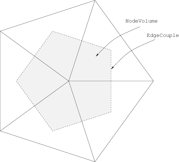
Fig. 4.1 Mesh elements in 2D.

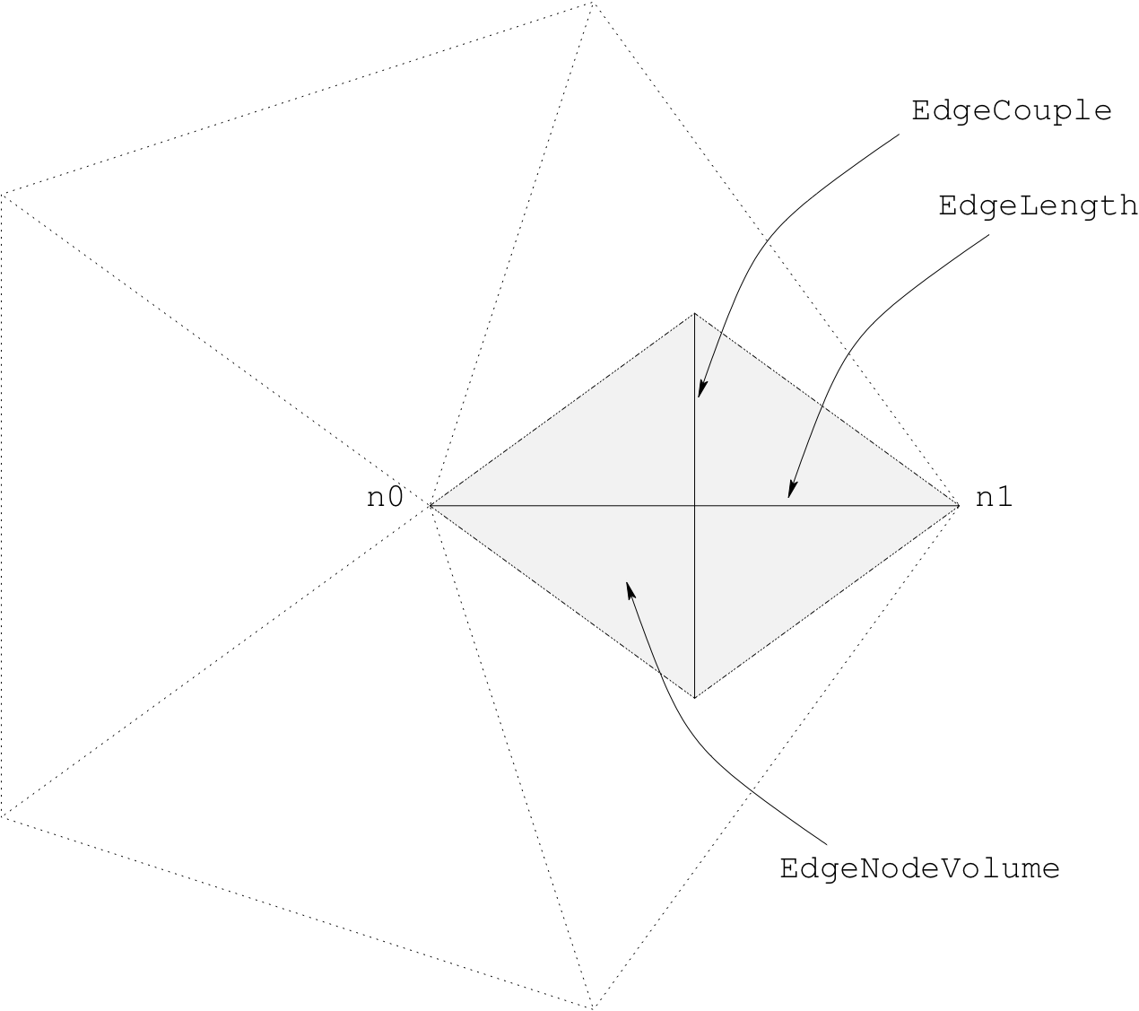
Fig. 4.2 Edge model constructs in 2D.

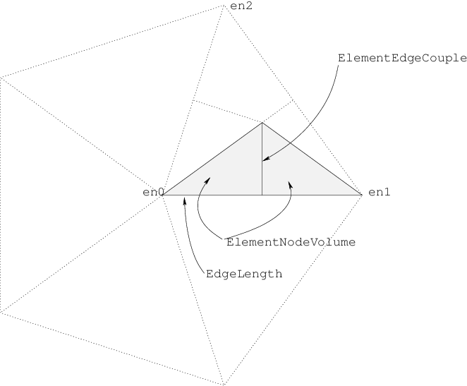
Fig. 4.3 Element edge model constructs in 2D.

In this form, we refer to a model integrated over the edges of triangles as edge models. Models integrated over the volume of each triangle vertex are referred to as node models. Element edge models are a special case where variables at other nodes off the edge may cause the flux to change.

There are a default set of models created in each region upon initialization of a device, and are typically based on the geometrical attributes. These are described in the following sections. Models required for describing the device behavior are created using the equation parser described in SYMDIFF. For special situations, custom matrix assembly is also available and is discussed in Custom Matrix assembly.

4.2. Bulk models

4.2.1. Node models

Node models may be specified in terms of other node models, mathematical functions, and parameters on the device. The simplest model is the node solution, and it represents the solution variables being solved for. Node models automatically created for a region are listed in Table 4.1.

In this example, we present an implementation of Shockley Read Hall recombination [5].

USRH="-ElectronCharge*(Electrons*Holes - n_i^2)/(taup*(Electrons + n1) \
         + taun*(Holes + p1))")
dUSRHdn="simplify(diff(%s, Electrons))" % USRH
dUSRHdp="simplify(diff(%s, Holes))" % USRH
devsim.node_model(device='MyDevice', region='MyRegion',
  name="USRH", equation=USRH)
devsim.node_model(device='MyDevice', region='MyRegion',
  name="USRH:Electrons", equation=dUSRHdn)
devsim.node_model(device='MyDevice', region='MyRegion',
  name="USRH:Holes", equation=dUSRHdp)

The first model specified, USRH, is the recombination model itself. The derivatives with respect to electrons and holes are USRH:Electrons and USRH:Holes, respectively. In this particular example Electrons and Holes have already been defined as solution variables. The remaining variables in the equation have already been specified as parameters.

The diff function tells the equation parser to take the derivative of the original expression, with respect to the variable specified as the second argument. During equation assembly, these derivatives are required in order to converge upon a solution. The simplify function tells the expression parser to attempt to simplify the expression as much as possible.

Table 4.1 Node models defined on each region of a device.

Node Model	Description
AtContactNode	Evaluates to 1 if node is a contact node, otherwise 0
NodeVolume	The volume of the node. Used for volume integration of node models on nodes in mesh
NSurfaceNormal_x	The surface normal to points on the interface or contact (2D and 3D)
NSurfaceNormal_y	The surface normal to points on the interface or contact (2D and 3D)
NSurfaceNormal_z	The surface normal to points on the interface or contact (3D)
SurfaceArea	The surface area of a node on interface nodes, otherwise 0
ContactSurfaceArea	The surface area of a node on contact nodes, otherwise 0
coordinate_index	Coordinate index of the node on the device
node_index	Index of the node in the region
x	x position of the node
y	y position of the node
z	z position of the node

4.2.2. Edge models

Edge models may be specified in terms of other edge models, mathematical functions, and parameters on the device. In addition, edge models may reference node models defined on the ends of the edge. As depicted in Fig. 4.2, edge models are with respect to the two nodes on the edge, n0 and n1.

For example, to calculate the electric field on the edges in the region, the following scheme is employed:

devsim.edge_model(device="device", region="region", name="ElectricField",
           equation="(Potential@n0 - Potential@n1)*EdgeInverseLength")
devsim.edge_model(device="device", region="region",
           name="ElectricField:Potential@n0", equation="EdgeInverseLength")
devsim.edge_model(device="device", region="region",
           name="ElectricField:Potential@n1", equation="-EdgeInverseLength")

In this example, EdgeInverseLength is a built-in model for the inverse length between nodes on an edge. Potential@n0 and Potential@n1 is the Potential node solution on the nodes at the end of the edge. These edge quantities are created using the devsim.edge_from_node_model(). In addition, the devsim.edge_average_model() can be used to create edge models in terms of node model quantities.

Edge models automatically created for a region are listed in Table 4.2.

Table 4.2 Edge models defined on each region of a device.

Edge Model	Description
EdgeCouple	The length of the perpendicular bisector of an element edge. Used to perform surface integration of edge models on edges in mesh.
EdgeNodeVolume	The volume for each node on an edge. Used to perform volume integration of edge models on edges in mesh.
EdgeInverseLength	Inverse of the EdgeLength.
EdgeLength	The distance between the two nodes of an edge
edge_index	Index of the edge on the region
unitx	x component of the unit vector along an edge
unity	y component of the unit vector along an edge (2D and 3D)
unitz	z component of the unit vector along an edge (3D only)

4.2.3. Element edge models

Element edge models are used when the edge quantitites cannot be specified entirely in terms of the quantities on both nodes of the edge, such as when the carrier mobility is dependent on the normal electric field. In 2D, element edge models are evaluated on each triangle edge. As depicted in Fig. 4.3, edge models are with respect to the three nodes on each triangle edge and are denoted as en0, en1, and en2. Derivatives are with respect to each node on the triangle.

In 3D, element edge models are evaluated on each tetrahedron edge. Derivatives are with respect to the nodes on both triangles on the tetrahedron edge. Element edge models automatically created for a region are listed in Table 4.3.

As an alternative to treating integrating the element edge model with respect to ElementEdgeCouple, the integration may be performed with respect to ElementNodeVolume. See devsim.equation() for more information.

Table 4.3 Element edge models defined on each region of a device.

Element Edge Model	Description
ElementEdgeCouple	The length of the perpendicular bisector of an edge. Used to perform surface integration of element edge model on element edge in the mesh.
ElementNodeVolume	The node volume at either end of each element edge.

4.2.4. Model derivatives

To converge upon the solution, derivatives are required with respect to each of the solution variables in the system. DEVSIM will look for the required derivatives. For a model model, the derivatives with respect to solution variable variable are presented in Table 4.4.

Table 4.4 Required derivatives for equation assembly. model is the name of the model being evaluated, and variable is one of the solution variables being solved at each node.

Model Type	Derivatives Required
Node Model	model:variable
Edge Model	model:variable@n0, model:variable@n1
Element Edge Model	model:variable@en0, model:variable@en1, model:variable@en2, model:variable@en3 (3D)

4.2.5. Conversions between model types

The devsim.edge_from_node_model() is used to create edge models referring to the nodes connecting the edge. For example, the edge models Potential@n0 and Potential@n1 refer to the Potential node model on each end of the edge.

The devsim.edge_average_model() creates an edge model which is either the arithmetic mean, geometric mean, gradient, or negative of the gradient of the node model on each edge.

When an edge model is referred to in an element edge model expression, the edge values are implicity converted into element edge values during expression evaluation. In addition, derivatives of the edge model with respect to the nodes of an element edge are required, they are converted as well. For example, edgemodel:variable@n0 and edgemodel:variable@n1 are implicitly converted to edgemodel:variable@en0 and edgemodel:variable@en1, respectively.

The devsim.element_from_edge_model() is used to create directional components of an edge model over an entire element. The derivative option is used with this command to create the derivatives with respect to a specific node model. The devsim.element_from_node_model() is used to create element edge models referring to each node on the element of the element edge.

4.2.6. Equation assembly

Bulk equations are specified in terms of the node, edge, and element edge models using the devsim.equation(). Node models are integrated with respect to the node volume. Edge models are integrated with the perpendicular bisectors along the edge onto the nodes on either end.

Element edge models are treated as flux terms and are integrated with respect to ElementEdgeCouple using the element_model option. Alternatively, they may be treated as source terms and are integrated with respect to ElementNodeVolume using the volume_node0_model and volume_node1_model option.

In this example, we are specifying the Potential Equation in the region to consist of a flux term named PotentialEdgeFlux and to not have any node volume terms.

devsim.equation(device="device", region="region", name="PotentialEquation",
  variable_name="Potential", edge_model="PotentialEdgeFlux",
  variable_update="log_damp" )

In addition, the solution variable coupled with this equation is Potential and it will be updated using logarithmic damping.

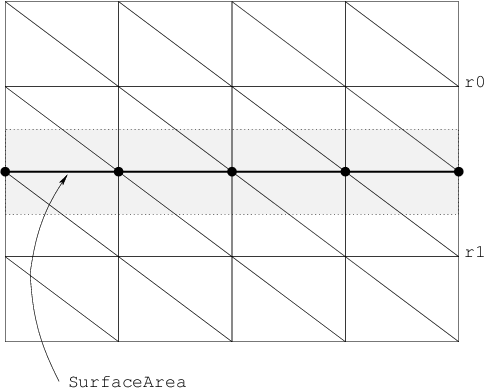
Fig. 4.4 Interface constructs in 2D. Interface node pairs are located at each \(\bullet\). The SurfaceArea model is used to integrate flux term models.

Table 4.5 Required derivatives for interface equation assembly. The node model name nodemodel and its derivatives nodemodel:variable are suffixed with @r0 and @r1 to denote which region on the interface is being referred to.

Model Type	Model Name	Derivatives Required
Node Model (region 0)	nodemodel@r0	nodemodel:variable@r0
Node Model (region 1)	nodemodel@r1	nodemodel:variable@r1
Interface Node Model	inodemodel	inodemodel:variable@r0, inodemodel:variable@r1

4.3. Interface

4.3.1. Interface models

Fig. 4.4 depicts an interface in DEVSIM. It is a collection of overlapping nodes existing in two regions, r0 and r1.

Interface models are node models specific to the interface being considered. They are unique from bulk node models, in the sense that they may refer to node models on both sides of the interface. They are specified using the devsim.interface_model(). Interface models may refer to node models or parameters on either side of the interface using the syntax nodemodel@r0 and nodemodel@r1 to refer to the node model in the first and second regions of the interface. The naming convention for node models, interface node models, and their derivatives are shown in Table 4.5.

devsim.interface_model(device="device", interface="interface",
  name="continuousPotential", equation="Potential@r0-Potential@r1")

4.3.2. Interface model derivatives

For a given interface model, model, the derivatives with respect to the variable variable in the regions are

• model:variable@r0

• model:variable@r1

devsim.interface_model(device="device", interface="interface",
  name="continuousPotential:Potential@r0", equation="1")
devsim.interface_model(device="device", interface="interface",
  name="continuousPotential:Potential@r1", equation="-1")

4.3.3. Interface equation assembly

There are three types of interface equations considered in DEVSIM. They are both activated using the devsim.interface_equation().

In the first form, continuous, the equations for the nodes on both sides of the interface are integrated with respect to their volumes and added into the same equation. An additional equation is then specified to relate the variables on both sides. In this example, continuity in the potential solution across the interface is enforced, using the continuousPotential model defined in the previous section.

devsim.interface_equation(device="device", interface="interface", name="PotentialEquation",
                interface_model="continuousPotential", type="continuous")

In the second form, fluxterm, a flux term is integrated over the surface area of the interface and added to the first region, and subtracted from the second.

In the third form, hybrid, equations for nodes on both sides of the interface are added into the equation for the node in the first region. The equation for the node on the second interface is integrated in the second region, and the fluxterm is subracted in the second region.

4.4. Contact

Fig. 4.5 Contact constructs in 2D.

4.4.1. Contact models

Fig. 4.5 depicts how a contact is treated in a simulation. It is a collection of nodes on a region. During assembly, the specified models form an equation, which replaces the equation applied to these nodes for a bulk node.

Contact models are equivalent to node and edge models, and are specified using the devsim.contact_node_model() and the devsim.contact_edge_model(), respectively. The key difference is that the models are only evaluated on the contact nodes for the contact specified.

4.4.2. Contact model derivatives

The derivatives are equivalent to the discussion in Model derivatives. If external circuit boundary conditions are being used, the model model derivative with respect to the circuit node node name should be specified as model:node.

4.4.3. Contact equation assembly

The devsim.contact_equation() is used to specify the boundary conditions on the contact nodes. The models specified replace the models specified for bulk equations of the same name. For example, the node model specified for the contact equation is assembled on the contact nodes, instead of the node model specified for the bulk equation. Contact equation models not specified are not assembled, even if the model exists on the bulk equation for the region attached to the contact.

As an example

devsim.contact_equation(device="device", contact="contact", name="PotentialEquation",
  node_model="contact_bc", edge_charge_model="DField")

Current models refer to the instantaneous current flowing into the device. Charge models refer to the instantaneous charge at the contact.

During a transient, small-signal or ac simulation, the time derivative is taken so that the net current into a circuit node is

\[I\left(t\right) = i\left(t\right) + \frac{\partial q \left(t\right)}{\partial t}\]

where \(i\) is the integrated current and \(q\) is the integrated charge.

4.5. Custom Matrix assembly

The devsim.custom_equation() command is used to register callbacks to be called during matrix and right hand side assembly. The Python procedure should expect to receive two arguments and return two lists and a boolean value. For example a procedure named myassemble registered with

devsim.custom_equation(name="test1", procedure="myassemble")

expects two arguments

def myassemble(what, timemode):
  .
  .
  .
  return rcv, rv, True

where what may be passed as one of

MATRIXONLY

RHS

MATRIXANDRHS

and timemode may be passed as one of

DC

TIME

When timemode is DC, the time-independent part of the equation is returned. When timemode is TIME, the time-derivative part of the equation is returned. The simulator will scale the time-derivative terms with the proper frequency or time scale.

The return value from the procedure must return two lists and a boolean value of the form

[1 1 1.0 2 2 1.0 1 2 -1.0 2 1 -1.0 2 2 1.0], [1 1.0 2 1.0 2 -1.0], True

where the length of the first list is divisible by 3 and contains the row, column, and value to be assembled into the matrix. The second list is divisible by 2 and contains the right hand side entries. Either list may be empty.

The boolean value denotes whether the matrix and right hand side entries should be row permutated. A value of True should be used for assembling bulk equations, and a value of False should be used for assembling contact and interface boundary conditions.

The devsim.get_circuit_equation_number() may be used to get the equation numbers corresponding to circuit node names. The devsim.get_equation_numbers() may be used to find the equation number corresponding to each node index in a region.

The matrix and right hand side entries should be scaled by the NodeVolume if they are assembled into locations in a device region as volume integration.

4.6. Cylindrical Coordinate Systems

In 2D, models representing the edge couples, surface areas and node volumes may be generated using the following commands:

• devsim.cylindrical_edge_couple()

• devsim.cylindrical_node_volume()

• devsim.cylindrical_surface_area()

In order to change the integration from the default models to cylindrical models, the following parameters may be set

set_parameter(name="node_volume_model",
  value="CylindricalNodeVolume")
set_parameter(name="edge_couple_model",
  value="CylindricalEdgeCouple")
set_parameter(name="edge_node0_volume_model",
  value="CylindricalEdgeNodeVolume@n0")
set_parameter(name="edge_node1_volume_model",
  value="CylindricalEdgeNodeVolume@n1")
set_parameter(name="element_edge_couple_model",
  value="ElementCylindricalEdgeCouple")
set_parameter(name="element_node0_volume_model",
  value="ElementCylindricalNodeVolume@en0")
set_parameter(name="element_node1_volume_model",
  value="ElementCylindricalNodeVolume@en1")