13. Simple Examples

13.1. Capacitor

13.1.1. Overview

In this chapter, we present a capacitance simulations. The purpose is to demonstrate the use of DEVSIM with a rather simple example. The first example in 1D capacitor is called cap1d.py and is located in the examples/capacitance directory distributed with DEVSIM. In this example, we have manually taken the derivative expressions. In other examples, we will show use of SYMDIFF to create the derivatives in an automatic fashion. The second example is in 2D capacitor.

13.1.2. 1D capacitor

Equations

In this example, we are solving Poisson’s equation. In differential operator form, the equation to be solved over the structure is:

\[\epsilon \nabla^2 \psi = 0\]

and the contact boundary equations are

\[\psi_i - V_{c} = 0\]

where \(\psi_i\) is the potential at the contact node and \(V_{c}\) is the applied voltage.

Creating the mesh

The following statements create a one-dimensional mesh which is \(1\) cm long with a \(0.1\) cm spacing. A contact is placed at \(0\) and \(1\) and are named contact1 and contact2 respectively.

from devsim import *
device="MyDevice"
region="MyRegion"

###
### Create a 1D mesh
###
create_1d_mesh (mesh="mesh1")
add_1d_mesh_line (mesh="mesh1", pos=0.0, ps=0.1, tag="contact1")
add_1d_mesh_line (mesh="mesh1", pos=1.0, ps=0.1, tag="contact2")
add_1d_contact   (mesh="mesh1", name="contact1", tag="contact1",
  material="metal")
add_1d_contact   (mesh="mesh1", name="contact2", tag="contact2",
  material="metal")
add_1d_region    (mesh="mesh1", material="Si", region=region,
  tag1="contact1", tag2="contact2")
finalize_mesh (mesh="mesh1")
create_device (mesh="mesh1", device=device)

Setting device parameters

In this section, we set the value of the permittivity to that of SiO \(_\text{2}\).

###
### Set parameters on the region
###
set_parameter(device=device, region=region,
  name="Permittivity", value=3.9*8.85e-14)

Creating the models

Solving for the Potential, \(\psi\), we first create the solution variable.

###
### Create the Potential solution variable
###
node_solution(device=device, region=region, name="Potential")

In order to create the edge models, we need to be able to refer to Potential on the nodes on each edge.

###
### Creates the Potential@n0 and Potential@n1 edge model
###
edge_from_node_model(device=device, region=region, node_model="Potential")

We then create the ElectricField model with knowledge of Potential on each node, as well as the EdgeInverseLength of each edge. We also manually calculate the derivative of ElectricField with Potential on each node and name them ElectricField:Potential@n0 and ElectricField:Potential@n1.

###
### Electric field on each edge, as well as its derivatives with respect to
### the potential at each node
###
edge_model(device=device, region=region, name="ElectricField",
                 equation="(Potential@n0 - Potential@n1)*EdgeInverseLength")

edge_model(device=device, region=region, name="ElectricField:Potential@n0",
                 equation="EdgeInverseLength")

edge_model(device=device, region=region, name="ElectricField:Potential@n1",
                 equation="-EdgeInverseLength")

We create DField to account for the electric displacement field.

###
### Model the D Field
###
edge_model(device=device, region=region, name="DField",
           equation="Permittivity*ElectricField")

edge_model(device=device, region=region, name="DField:Potential@n0",
           equation="diff(Permittivity*ElectricField, Potential@n0)")

edge_model(device=device, region=region, name="DField:Potential@n1",
           equation="-DField:Potential@n0")

The bulk equation is now created for the structure using the models and parameters we have previously defined.

###
### Create the bulk equation
###
equation(device=device, region=region, name="PotentialEquation",
  variable_name="Potential", edge_model="DField",
  variable_update="default")

Contact boundary conditions

We then create the contact models and equations. We use the Python for loop construct and variable substitutions to create a unique model for each contact, contact1_bc and contact2_bc.

###
### Contact models and equations
###
for c in ("contact1", "contact2"):
  contact_node_model(device=device, contact=c, name="%s_bc" % c,
           equation="Potential - %s_bias" % c)

  contact_node_model(device=device, contact=c, name="%s_bc:Potential" % c,
             equation="1")

  contact_equation(device=device, contact=c, name="PotentialEquation",
             node_model="%s_bc" % c, edge_charge_model="DField")

In this example, the contact bias is applied through parameters named contact1_bias and contact2_bias. When applying the boundary conditions through circuit nodes, models with respect to their names and their derivatives would be required.

Setting the boundary conditions

###
### Set the contact
###
set_parameter(device=device, region=region, name="contact1_bias", value=1.0e-0)
set_parameter(device=device, region=region, name="contact2_bias", value=0.0)

###
### Solve
###
solve(type="dc", absolute_error=1.0, relative_error=1e-10, maximum_iterations=30)

###
### Print the charge on the contacts
###
for c in ("contact1", "contact2"):
  print("contact: %s charge: %1.5e"
    % (c, get_contact_charge(device=device, contact=c, equation="PotentialEquation")))

Running the simulation

We run the simulation and see the results.

contact2
 (region: MyRegion)
 (contact: contact1)
 (contact: contact2)
Region "MyRegion" on device "MyDevice" has equations 0:10
Device "MyDevice" has equations 0:10
number of equations 11
Iteration: 0
  Device: "MyDevice"  RelError: 1.00000e+00   AbsError: 1.00000e+00
    Region: "MyRegion"        RelError: 1.00000e+00   AbsError: 1.00000e+00
      Equation: "PotentialEquation"   RelError: 1.00000e+00   AbsError: 1.00000e+00
Iteration: 1
  Device: "MyDevice"  RelError: 2.77924e-16   AbsError: 1.12632e-16
    Region: "MyRegion"        RelError: 2.77924e-16   AbsError: 1.12632e-16
      Equation: "PotentialEquation"   RelError: 2.77924e-16   AbsError: 1.12632e-16
contact: contact1 charge: 3.45150e-13
contact: contact2 charge: -3.45150e-13

Which corresponds to our expected result of \(3.4515 10^{-13}\) \(\text{F}/\text{cm}^2\) for a homogenous capacitor.

13.1.3. 2D capacitor

This example is called cap2d.py and is located in the examples/capacitance directory distributed with DEVSIM. This file uses the same physics as the 1D example, but with a 2D structure. The mesh is built using the DEVSIM internal mesher. An air region exists with two electrodes in the simulation domain.

Defining the mesh

from devsim import *
device="MyDevice"
region="MyRegion"

xmin=-25
x1  =-24.975
x2  =-2
x3  =2
x4  =24.975
xmax=25.0

ymin=0.0
y1  =0.1
y2  =0.2
y3  =0.8
y4  =0.9
ymax=50.0

create_2d_mesh(mesh=device)
add_2d_mesh_line(mesh=device, dir="y", pos=ymin, ps=0.1)
add_2d_mesh_line(mesh=device, dir="y", pos=y1  , ps=0.1)
add_2d_mesh_line(mesh=device, dir="y", pos=y2  , ps=0.1)
add_2d_mesh_line(mesh=device, dir="y", pos=y3  , ps=0.1)
add_2d_mesh_line(mesh=device, dir="y", pos=y4  , ps=0.1)
add_2d_mesh_line(mesh=device, dir="y", pos=ymax, ps=5.0)

device=device
region="air"

add_2d_mesh_line(mesh=device, dir="x", pos=xmin, ps=5)
add_2d_mesh_line(mesh=device, dir="x", pos=x1  , ps=2)
add_2d_mesh_line(mesh=device, dir="x", pos=x2  , ps=0.05)
add_2d_mesh_line(mesh=device, dir="x", pos=x3  , ps=0.05)
add_2d_mesh_line(mesh=device, dir="x", pos=x4  , ps=2)
add_2d_mesh_line(mesh=device, dir="x", pos=xmax, ps=5)

add_2d_region(mesh=device, material="gas"  , region="air", yl=ymin, yh=ymax, xl=xmin, xh=xmax)
add_2d_region(mesh=device, material="metal", region="m1" , yl=y1  , yh=y2  , xl=x1  , xh=x4)
add_2d_region(mesh=device, material="metal", region="m2" , yl=y3  , yh=y4  , xl=x2  , xh=x3)

# must be air since contacts don't have any equations
add_2d_contact(mesh=device, name="bot", region="air", material="metal", yl=y1, yh=y2, xl=x1, xh=x4)
add_2d_contact(mesh=device, name="top", region="air", material="metal", yl=y3, yh=y4, xl=x2, xh=x3)
finalize_mesh(mesh=device)
create_device(mesh=device, device=device)

Setting up the models

###
### Set parameters on the region
###
set_parameter(device=device, region=region, name="Permittivity", value=3.9*8.85e-14)

###
### Create the Potential solution variable
###
node_solution(device=device, region=region, name="Potential")

###
### Creates the Potential@n0 and Potential@n1 edge model
###
edge_from_node_model(device=device, region=region, node_model="Potential")

###
### Electric field on each edge, as well as its derivatives with respect to
### the potential at each node
###
edge_model(device=device, region=region, name="ElectricField",
                 equation="(Potential@n0 - Potential@n1)*EdgeInverseLength")

edge_model(device=device, region=region, name="ElectricField:Potential@n0",
                 equation="EdgeInverseLength")

edge_model(device=device, region=region, name="ElectricField:Potential@n1",
                 equation="-EdgeInverseLength")

###
### Model the D Field
###
edge_model(device=device, region=region, name="DField",
           equation="Permittivity*ElectricField")

edge_model(device=device, region=region, name="DField:Potential@n0",
           equation="diff(Permittivity*ElectricField, Potential@n0)")

edge_model(device=device, region=region, name="DField:Potential@n1",
           equation="-DField:Potential@n0")

###
### Create the bulk equation
###
equation(device=device, region=region, name="PotentialEquation",
  variable_name="Potential", edge_model="DField",
  variable_update="default")


###
### Contact models and equations
###
for c in ("top", "bot"):
  contact_node_model(device=device, contact=c, name="%s_bc" % c,
           equation="Potential - %s_bias" % c)

  contact_node_model(device=device, contact=c, name="%s_bc:Potential" % c,
             equation="1")

  contact_equation(device=device, contact=c, name="PotentialEquation",
             node_model="%s_bc" % c, edge_charge_model="DField")

###
### Set the contact
###
set_parameter(device=device, name="top_bias", value=1.0e-0)
set_parameter(device=device, name="bot_bias", value=0.0)



edge_model(device=device, region="m1", name="ElectricField", equation="0")
edge_model(device=device, region="m2", name="ElectricField", equation="0")
node_model(device=device, region="m1", name="Potential", equation="bot_bias;")
node_model(device=device, region="m2", name="Potential", equation="top_bias;")


solve(type="dc", absolute_error=1.0, relative_error=1e-10, maximum_iterations=30,
  solver_type="direct")

Fields for visualization

Before writing the mesh out for visualization, the element_from_edge_model is used to calculate the electric field at each triangle center in the mesh. The components are the ElectricField_x and ElectricField_y.

element_from_edge_model(edge_model="ElectricField", device=device, region=region)
print(get_contact_charge(device=device, contact="top", equation="PotentialEquation"))
print(get_contact_charge(device=device, contact="bot", equation="PotentialEquation"))

write_devices(file="cap2d.msh", type="devsim")
write_devices(file="cap2d.dat", type="tecplot")

Running the simulation

Creating Region air
Creating Region m1
Creating Region m2
Adding 8281 nodes
Adding 23918 edges with 22990 duplicates removed
Adding 15636 triangles  with 0 duplicate removed
Adding 334 nodes
Adding 665 edges with 331 duplicates removed
Adding 332 triangles  with 0 duplicate removed
Adding 162 nodes
Adding 321 edges with 159 duplicates removed
Adding 160 triangles  with 0 duplicate removed
Contact bot in region air with 334 nodes
Contact top in region air with 162 nodes
Region "air" on device "MyDevice" has equations 0:8280
Region "m1" on device "MyDevice" has no equations.
Region "m2" on device "MyDevice" has no equations.
Device "MyDevice" has equations 0:8280
number of equations 8281
Iteration: 0
  Device: "MyDevice"  RelError: 1.00000e+00   AbsError: 1.00000e+00
    Region: "air"     RelError: 1.00000e+00   AbsError: 1.00000e+00
      Equation: "PotentialEquation"   RelError: 1.00000e+00   AbsError: 1.00000e+00
Iteration: 1
  Device: "MyDevice"  RelError: 1.25144e-12   AbsError: 1.73395e-13
    Region: "air"     RelError: 1.25144e-12   AbsError: 1.73395e-13
      Equation: "PotentialEquation"   RelError: 1.25144e-12   AbsError: 1.73395e-13
3.35017166004e-12
-3.35017166004e-12

A visualization of the results is shown in Capacitance simulation result. The coloring is by Potential, and the stream traces are for components of ElectricField..

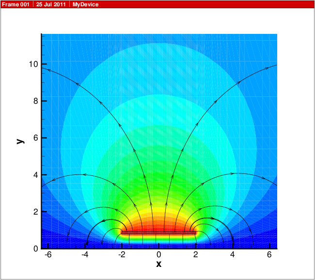
Fig. 13.1 Capacitance simulation result. The coloring is by Potential, and the stream traces are for components of ElectricField.

13.2. Diode

13.2.1. Overview

The diode examples are located in the examples/diode. They demonstrate the use of packages located in the python_packages directory to simulate drift-diffusion using the Scharfetter-Gummel method [9].

13.2.2. 1D diode

Using the python packages

For these examples, python modules are provided to supply the appropriate model and parameter settings. A listing is shown in Python package files. The devsim.python_packages module is part of the distribution. The example files in the DEVSIM distribution set the path properly when loading modules.

Table 13.1 Python package files

model_create	Creation of models and their derivatives
ramp	Ramping bias and automatic stepping
simple_dd	Functions for calculating bulk electron and hole current
simple_physics	Functions for setting up device physics

For this example, diode_1d.py, the following line is used to import the relevant physics.

from devsim import *
from simple_physics import *

Creating the mesh

This creates a mesh \(10^{-5}\) cm long with a junction located at the midpoint. The name of the device is MyDevice with a single region names MyRegion. The contacts on either end are called top and bot.

def createMesh(device, region):
  create_1d_mesh(mesh="dio")
  add_1d_mesh_line(mesh="dio", pos=0, ps=1e-7, tag="top")
  add_1d_mesh_line(mesh="dio", pos=0.5e-5, ps=1e-9, tag="mid")
  add_1d_mesh_line(mesh="dio", pos=1e-5, ps=1e-7, tag="bot")
  add_1d_contact  (mesh="dio", name="top", tag="top", material="metal")
  add_1d_contact  (mesh="dio", name="bot", tag="bot", material="metal")
  add_1d_region   (mesh="dio", material="Si", region=region, tag1="top", tag2="bot")
  finalize_mesh(mesh="dio")
  create_device(mesh="dio", device=device)

device="MyDevice"
region="MyRegion"

createMesh(device, region)

Physical models and parameters

####
#### Set parameters for 300 K
####
SetSiliconParameters(device, region, 300)
set_parameter(device=device, region=region, name="taun", value=1e-8)
set_parameter(device=device, region=region, name="taup", value=1e-8)

####
#### NetDoping
####
CreateNodeModel(device, region, "Acceptors", "1.0e18*step(0.5e-5-x)")
CreateNodeModel(device, region, "Donors",    "1.0e18*step(x-0.5e-5)")
CreateNodeModel(device, region, "NetDoping", "Donors-Acceptors")
print_node_values(device=device, region=region, name="NetDoping")

####
#### Create Potential, Potential@n0, Potential@n1
####
CreateSolution(device, region, "Potential")

####
#### Create potential only physical models
####
CreateSiliconPotentialOnly(device, region)

####
#### Set up the contacts applying a bias
####
for i in get_contact_list(device=device):
  set_parameter(device=device, name=GetContactBiasName(i), value=0.0)
  CreateSiliconPotentialOnlyContact(device, region, i)


####
#### Initial DC solution
####
solve(type="dc", absolute_error=1.0, relative_error=1e-12, maximum_iterations=30)

####
#### drift diffusion solution variables
####
CreateSolution(device, region, "Electrons")
CreateSolution(device, region, "Holes")

####
#### create initial guess from dc only solution
####
set_node_values(device=device, region=region,
  name="Electrons", init_from="IntrinsicElectrons")
set_node_values(device=device, region=region,
  name="Holes", init_from="IntrinsicHoles")

###
### Set up equations
###
CreateSiliconDriftDiffusion(device, region)
for i in get_contact_list(device=device):
  CreateSiliconDriftDiffusionAtContact(device, region, i)

###
### Drift diffusion simulation at equilibrium
###
solve(type="dc", absolute_error=1e10, relative_error=1e-10, maximum_iterations=30)

####
#### Ramp the bias to 0.5 Volts
####
v = 0.0
while v < 0.51:
  set_parameter(device=device, name=GetContactBiasName("top"), value=v)
  solve(type="dc", absolute_error=1e10, relative_error=1e-10, maximum_iterations=30)
  PrintCurrents(device, "top")
  PrintCurrents(device, "bot")
  v += 0.1

####
#### Write out the result
####
write_devices(file="diode_1d.dat", type="tecplot")

Plotting the result

A plot showing the doping profile and carrier densities are shown in Carrier density versus position in 1D diode.. The potential and electric field distribution is shown in Potential and electric field versus position in 1D diode.. The current distributions are shown in Electron and hole current and recombination..

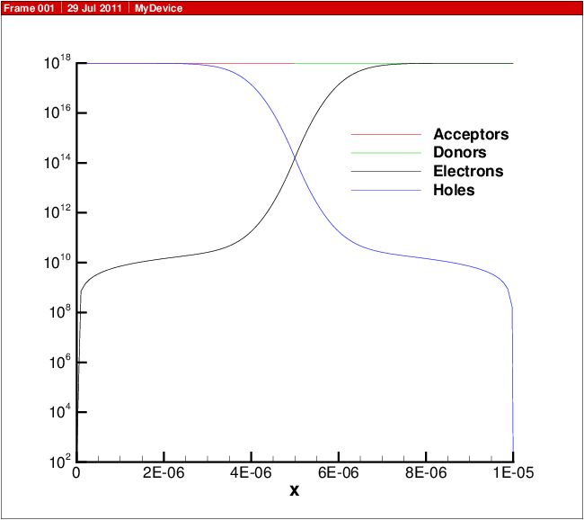
Fig. 13.2 Carrier density versus position in 1D diode.

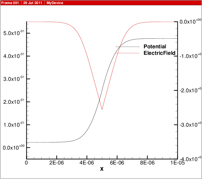
Fig. 13.3 Potential and electric field versus position in 1D diode.

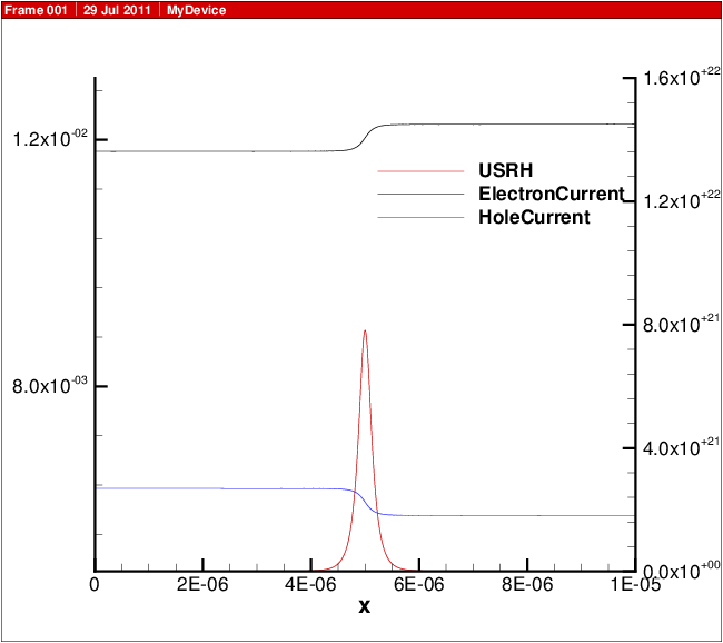
Fig. 13.4 Electron and hole current and recombination.